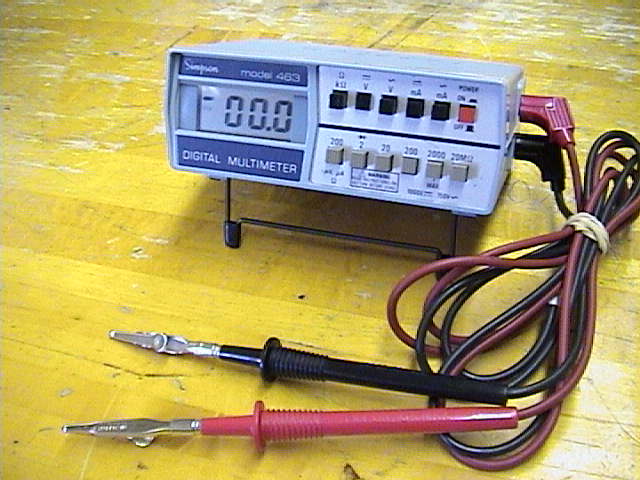
This laboratory experiment is designed to investigate the behavior of capacitor responses of RC circuits, the basis for most electronic timing circuits. An oscilloscope and digital multimeter will be used in this lab.

Capacitors in Series and Parallel

A capacitor is a common electronic circuit component that consists of two parallel plates separated by an insulating material called a dielectric. When a battery with voltage is connected across the capacitor, equal and opposite charges rapidly collect onto the plates due to the electric field created by the wires connecting the two plates¹. Once the plates are fully charged, one plate will have a net positive charge while the other plate will have a net negative charge . It has been shown empirically that the charge on one of the plates, , is directly proportional to the applied potential difference, , and the constant of proportionality is known as the capacitance², . The amount of charge on each plate in this steady-state is then written as

(1)

where is in coulombs, is in volts, and is in farads (after 19^th century British physicists Michael Faraday). That is, . A one-farad capacitor is physically quite large, so it is more common to see capacitors in the picofarad () to microfarad () range. Since the capacitor charges in some finite amount of time, the charge that exists on one of the plates at any time, that is before a steady-state exists, is given by

(2)

When capacitors are connected together in series and then connected to a battery, as shown in Figure 1, the same amount of charge must build up on each of the capacitors. It can be shown that the behavior of these capacitors is as if there was one single capacitor with an effective capacitance, , given by the following

Capacitors in series

(3)

It should be readily seen that the effective capacitance of capacitors in series is smaller than the capacitance of any of the contributing elements. However when capacitors are connected in parallel, as shown in Figure 2, the effective capacitance is given by the sum of each capacitance, or

Capacitors in parallel

(4)

Figure 1. Capacitors in series.		Figure 2. Capacitors in parallel.

Behavior of an RC Circuit

Figure 3. Schematic of an RC circuit. The components in the dotted box are analogous to a square-wave generator with outputs at points and . The switch continuously moves between points and creating a square wave as shown in Figure 4a.

Suppose we connect a battery, with voltage, , across a resistor and capacitor in series as shown by Figure 3. This is commonly known as an RC circuit and is used often in electronic timing circuits. When the switch is moved to position , the battery is connected to the circuit and a time-varying current begins flowing through the circuit as the capacitor charges. When the switch is then moved to position , the battery is taken out of the circuit and the capacitor discharges through the resistor. If the switch is moved alternately between positions and , the voltage across points and can be plotted and would resemble Figure 4.

Figure 4. A voltage pattern known as a square wave. Moving the switch in Figure 3 alternatively between positions and can produce this voltage pattern. When the switch is in position , the input voltage is the peak voltage is . When the switch is moves to position , the input voltage drops to zero. A function generator more commonly produces square-wave voltages.

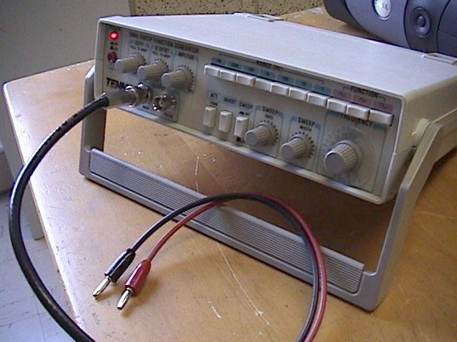
This voltage pattern is known as a square wave, for obvious reasons, and is commonly produced by a function generator. The function generator is capable of producing voltages that behave like a sine, square or saw-tooth functions. Additionally, the frequency of the wave may be varied with the function generator. The dotted-box in Figure 3 may be thought of as a function generator with points and as outputs.

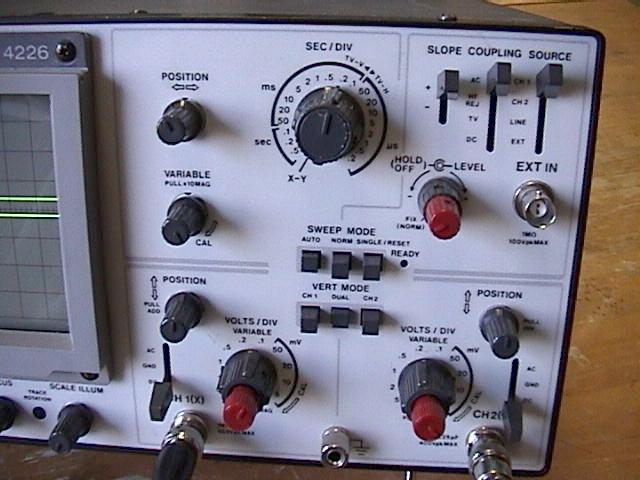
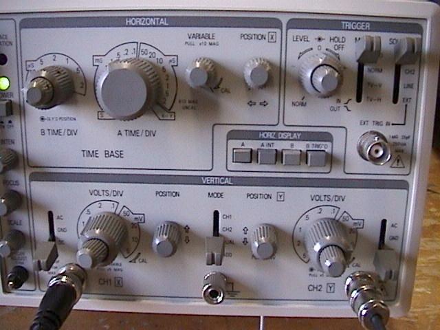
We will use a two-channel oscilloscope to monitor the important voltages throughout the experiment. An oscilloscope is an invaluable tool for testing electronic circuits by measuring voltages over time, and Figure 5 shows the schematic for monitoring an RC circuit with an oscilloscope. As shown in the figure below, the input voltage from the square-wave generator is monitored by channel one (CH 1) and the voltage across the capacitor is monitored by channel two (CH 2).

Figure 5. The RC circuit diagram. The oscilloscope's Channel 1 monitors the function generator while Channel 2 monitors the voltage drop across the capacitor.

The capacitor responds to the square-wave voltage input by going through a process of charging and discharging. It is shown below that during the charging cycle, the voltage across the capacitor is (see Equation 11 and Figure 6a below). When the switch is in position , the square-wave generator outputs a zero voltage and the capacitor discharges. It can also be shown that during the discharging cycle, the voltage across the capacitor is (see Equation 14 and Figure 6a below).

Circuit designers must be careful to ensure that the period of the square wave gives sufficient time for the capacitor to fully charge and discharge. It can be shown³ that, as a general rule of thumb, the time necessary for the capacitor of an RC circuit to nearly completely charge to , or discharge to zero, is .

Here it should be noted that the product is known as the time constant, , and has units of time⁴. The time constant is the characteristic time of the charging and discharging behavior of an RC circuit and represents the time it takes the current to decrease to of its initial value, whether the capacitor is charging or discharging. Over the period of one , the voltage across the charging capacitor increases by a factor of (see Equation 11). Conversely the voltage across the discharging capacitor decreases by a factor of over the same period, (see Equation 14). Put another way, in the voltage across a charging capacitor grows to 63.2% of its maximum voltage, , and in the voltage across a discharging capacitor shrinks to 36.8% of .

Figure 6a. The square wave that drives the RC circuit. When the switch in Figure 3 is in position , the input voltage is the peak voltage is . When the switch is moves to position , the input voltage drops to zero. In this experiment, this input voltage is read by the oscilloscope's CH 1.		Figure 6b. The voltage drop across the capacitor of Figure 3 as read by the oscilloscope's CH 2. The capacitor alternately charges toward and discharges toward zero according to the input voltage shown in Figure 6a. Here, the frequency (and therefore period) of the input square wave voltage is exactly such that the capacitor is allowed to fully charge and discharge. The time constant, , is equivalent to , and is defined by Equations 11 or 14.

A Charging Capacitor of an RC Circuit

Say a square-wave voltage, like the one in Figure 6a, is applied across an RC circuit. If one were to continually monitor the voltage across the capacitor, the waveform would resemble that of Figure 6b. Note that when the switch is in position , the square-wave generator outputs a voltage and the capacitor charges. Using Kirchhoff's rules we can examine the voltage drop across each circuit component while the capacitor is charging,

(5)

where is the battery voltage, is the voltage drop across the resistor (according to Ohm's law), and is the voltage drop across the capacitor (from Equation 2). (To simplify the notation, the time dependence of the current and charge will be dropped from our notation from here on.)

Substituting in Equation 5 and rearranging the equation, we can show

(6)

Integrating this equation and applying the initial condition at , Equation 6 can be written⁵

(7)

Evaluating the integrals we find

(8)

It can be shown⁶ that Equation 8 simplifies to

Charge as capacitor charges

(9)

where is the base of the natural logarithm. If we let and differentiate Equation 9, we find⁷ the current in our circuit to be

Current as capacitor charges

(10)

Using Equations 2 and 9, we find⁸ the voltage drop across the capacitor as it charges to be

Voltage across charging capacitor

(11)

Note that as , approaches , becomes , and approaches 0. In other words, as the capacitor charges, its voltage approaches the battery voltage and the charge on the capacitor plates approaches the steady-state condition () as time increases as shown in Figure 6b. The current approaches zero as the steady-state condition is realized.

A Discharging Capacitor of an RC Circuit

With similar arguments we can determine the behavior of the capacitor when it discharges. If we now move the switch in Figure 3 to position , the battery is removed from the circuit and the capacitor will begin discharging. Applying Kirchhoff's law to the new circuit with an initial condition of when , we can examine the charge, current and capacitor voltage as the capacitor discharges. It is left as an exercise to derive the following equations:

Charge as capacitor discharges

(12)

Current as capacitor discharges

(13)

Voltage across discharging capacitor

(14)

Note that as , , and all approach 0. In other words, as the capacitor discharges, its voltage, charge and current all approach zero as the capacitor returns to its initial state as shown in Figure 6b. As with the charging behavior of the capacitor, it is important to note that if the half-period of the input square wave voltage is less than ~, sufficient time will not exist for the capacitor to fully discharge! Again, proof of this is left as an exercise for the student.

Figure 7. A square wave with a longer period drives the RC circuit and the voltage response across the capacitor is slightly different than that shown in Figure 6b. It can be assumed that the circuits are the same for Figures 6 and 7. The capacitor charges in the same amount of time as the one shown in Figure 6b, but because the square-wave period is longer, the capacitor here remains charged until the input voltage drops once again to zero.

Finally it may be enlightening to examine the voltage response of the capacitor when the period of the input voltage is such that the capacitor has ample time to charge. This situation is shown in Figure 7. Note that here the capacitor remains fully charges as long as the input voltage is . If we assume that Figures 6b and 7 show responses of identical circuits (that is identical time constants) then observe that the time to charge and discharge in both figures are identical. The only difference is that in Figure 7 the capacitor becomes fully charged and remains charged for a period of time. In Figure 6b, the capacitor becomes fully charged and then immediately begins discharging. However it is important to note that if the half-period of the input square-wave voltage shown in Figure 6a is any amount less, then sufficient time will not exist for the capacitor to fully charge or discharge!

Footnotes

1. There is no conduction current, , flowing between the plates of the capacitor because the gap between the plates constitutes an open circuit. However, a displacement current, , does exist due to the changing electric field between the plates as the capacitor charges. This term can be found in the general form of Ampère's law (also known as Ampère-Maxwell law): .

2. The capacitance of the unit can be written where is the permitivity of the dielectric, is the surface area of one of the capacitor plates, and is the separation of the plates.

3. See Question 6 in the question section of this laboratory write-up.

4. See Question 5 in the question section of this laboratory write-up.

5. See Question 11 in the question section of this laboratory write-up.

6. See Question 12 in the question section of this laboratory write-up.

7. See Question 13 in the question section of this laboratory write-up.

8. See Question 14 in the question section of this laboratory write-up.

1. Become familiar with your oscilloscope. Your instructor will walk the entire class through this Objective and discuss with you the basic operations of an oscilloscope. You should know how to zero both channels of the oscilloscope and put two traces on the screen simultaneously. You should be able to adjust the vertical and horizontal position of the scope traces. You should also be able to use the oscilloscope to read voltages and times. You should read several voltages including a AA battery, a 9-volt battery and the oscilloscope's calibration output.

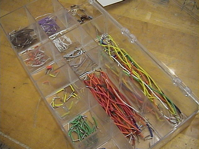
2. Use the function generator, breadboard, oscilloscope and any necessary wires to measure the frequency and amplitude of a ~100Hz sine wave at 25%-50% maximum amplitude. Repeat for a ~750Hz square wave.

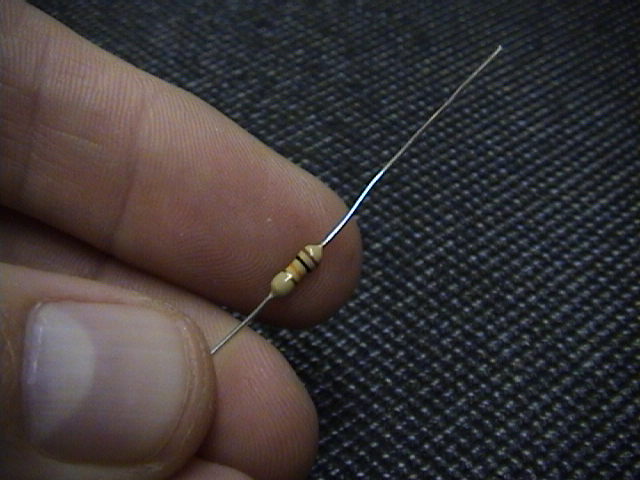
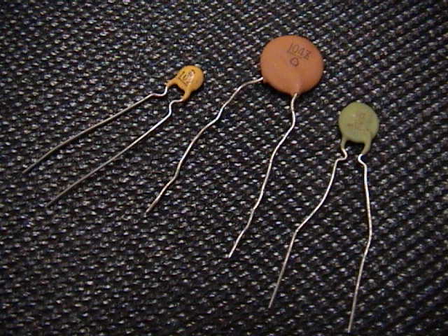
3. Use the resistor color code and the DMM to determine the value of the 10kW resistor. Note that the values of the three capacitors are as follows: Brown = 0.1mF, Green = 0.01mF, Yellow = 0.001mF. Determine the theoretical values for for three RC circuits using the resistor and the various capacitors.

4. Use the 0.1mF capacitor and the 10kW resistor and wire your breadboard according to Figure 5. Carefully adjust the frequency of the square wave and find the maximum frequency at which the capacitor will fully charge or discharge.

5. With the breadboard wired according to Objective 4, use the oscilloscope to determine the experimental time constant, , for the capacitor charging and discharging. (Hint: Calculate the capacitor voltage, , when .)

6. Use your breadboard to connect all three capacitors together in series. Then, use the 10kW resistor with the capacitors in series to form an RC circuit. Use the experimental apparatus and your knowledge of RC circuits to determine the effective capacitance, , of the capacitors in series.

7. Use your breadboard to connect all three capacitors together in parallel. Then, use the 10kW resistor with the capacitors in parallel to form an RC circuit. Use the experimental apparatus and your knowledge of RC circuits to determine the effective capacitance, , of the capacitors in parallel.

(Figure 8.) Capacitors of various capacitance values. (Figure 9.) The 10kW resistor. (Figure 10.) Digital Multi-meter or DMM may be used to measure resistance. (Figure 11.) The breadboard is used to connect circuit components. Notice the binding posts can be used to easily bring power from the function generator (Figure 14). You may find tutorials on using the breadboard in the On-line Assistance section. (Figure 12.) Jumper wires for use with the breadboard (Figure 11). Use the pliers (Figure 13) to insert these wires into the breadboard. (Figure 13.) Pliers should be used to insert resistors and jumper wires into the breadboard. (Figure 14.) The function generator is capable of producing sine, square and saw-tooth waves. (Figure 15.) Oscilloscopes displays input voltages from two channels over time. (Figure 16.) Here is a close-up of the Heath scope. Notice the location of all the switches. All variable knobs should be off, that is, "pushed in or clicked off". (Figure 17.) Here is a close-up of the Goldstar scope. Notice the location of all the switches. All variable knobs should be off, that is, "pushed in or clicked off". (Figure 18.) A sine wave output from a function generator as displayed by the oscilloscope. If the oscilloscope's vertical axis is set to 2 volts/div and 2 ms/div, what is the amplitude, period and frequency of the sine wave? (Figure 19.) A square wave output from a function generator as displayed by the oscilloscope. If the oscilloscope's vertical axis is set to 2 volts/div and 2 ms/div, what is the amplitude, period and frequency of the square wave? Banana wires

[Click on images to enlarge.] 8 9 10 11 12 13 14 15 16 17 18 19

1. Caution!!! Do not over-drive the function generator. Keep voltage amplitudes to 25-50% of maximum output.

2. Be careful when determining the period of a square wave.

1. The XYZ's of oscilloscope operation
2. A nice oscilloscope tutorial from Clemson's Bioengineering Department. (Must have Power Point installed on your computer!)
3. Resistor color codes explained
4. Resistor color code calculator -- very cool
5. Another color code calculator
6. How to use a breadboard
7. Another breadboard tutorial
8. Some common circuit symbols
9. Some more symbols
10. Using Excel

Each lab group should download the Lab Report Template and fill in the relevant information as you perform the experiment. Each person in the group should print-out the Questions section and answer them individually. Since each lab group will turn in an electronic copy of the lab report, be sure to rename the lab report template file. The naming convention is as follows:

For example the group at lab table #5 working on the Ideal Gas Law experiment would rename their template file as "5 Gas Law.doc".

These Nudge Questions are to be answered by your group and checked by your TA as you do the lab. They should be answered in your lab notebook.

General Nudges

1. What are the possible units of amplitude as measured by the oscilloscope?
2. What are the possible units of time as measured by the oscilloscope?

1. Can you use the scope to monitor your heart rate in beats per second? That is, can you use the scope as a timing device?
2. What were the voltage of your batteries? Was this expected?
3. What type of output was given by the scope's output calibration?
4. What was the calibration voltage's period and amplitude?

1. What oscilloscope channel are you using?
2. What are the amplitudes of the waves?
3. What are the periods of the waves?

1. How does the color code reading compare to a DMM reading of resistance?
2. What are the units of ?
3. Which combination of R and C will require the most time for the capacitor to charge?
4. How does the time to charge the capacitor compare with the time to discharge it?

1. Using the oscilloscope, what is the value of the frequency that you using for this Objective? How does this compare to the dial reading of the function generator?
2. What is each channel of the scope monitoring?
3. Will the capacitor ever fully charge?
4. Is the time for the capacitor to approximately fully charge ?
5. What happens to the behavior of the capacitor voltage as the frequency is varied? Can you explain this?

1. What is the definition of the time constant, ?
2. How is measured?
3. How do your values for compare to your theoretical value?

1. What should the theoretical value of be?
2. What are the parameters of the input signal of your circuit? (E.g., what is the shape, amplitude, frequency of your input wave?)
3. How do you take the voltage across three capacitors in series?
4. What is the measured time constant, , for this circuit?
5. Does the theoretical value of agree with your experimental value?

1. What should the theoretical value of be?
2. What are the parameters of the input signal of your circuit? (E.g., what is the shape, amplitude, frequency of your input wave?)
3. How do you take the voltage across three capacitors in parallel?
4. What is the measured time constant, , for this circuit?
5. Does the theoretical value of agree with your experimental value?

These Questions are also found in the lab write-up template. They must be answered by each individual of the group. This is not a team activity. Each person should attach their own copy to the lab report just prior to handing in the lab to your TA.

1. i. What quantities can be measured by an oscilloscope?

   ii. The frequency and period of a sine wave are measured in what units?

2. Show that has units of time. Recall and .

3. Use Equations 2 and 9 to show that the voltage across capacitor is while the capacitor is charging.

4. i. Show that,the time necessary for the capacitor of an circuit to charge to 98 % of the input voltage or discharge to 2 % of the input voltage is ~ . You can show this theoretically using Equations 11 and 14.

   ii. Is the characteristic time constant the same when the capacitor is charging and when it is discharging?

5. Describe the voltage response of the capacitor of an circuit to a square wave whose half-period is

   i. Significantly smaller than .

   ii. Significantly greater than .

6. A square wave is input into an RC circuit allowing the capacitor to charge and discharge. The input voltage, , and capacitor voltage, , are shown below in the left image. How would the input frequency need to be changed to get to look like the image on the right? Can you think of two other ways to alter the circuit that would cause to look like the right image?
    
   [Click on images to enlarge them]

• You should work closely with students on Objective 1. Students have a very difficult time using the oscilloscope for the first time. Perhaps you should view Objective 1 as an activity that will be lead by the TA in which the entire class will follow, step-by-step.
• The calibration outputs for the oscilloscopes are as follows:
  • Heath: 2.0V peak-to-peak, ~0.96ms period.
  • Goldstar: 0.5v peak-to-peak, 1.0ms period.

As of now, there are no CUPOL experiments associated with this experiment.